Gaussian Test Case

You must have already downloaded and installed Polyphemus to have this test case working.

This test-case is up-to-date with the version 1.11.1 of Polyphemus. Below, [version] will stand for the version number you are using.

Note that a more complete and detailed version of this documentation is available in Polyphemus User's Guide although this should be sufficient to get the simulation running.

Step 1: Obtaining and Installing the Test Case

Download the file TestCase-Gaussian-1.11.1.tar.bz2. To uncompress this file, execute the following command:

$ tar xjvf TestCase-Gaussian-1.11.1.tar.bz2

This create a directory TestCase-Gaussian/ (referred to below as TestCase/), containing:

A subdirectory config/ which holds all the configuration files used in the preprocessing and the simulation. It is the directory from which to work.
A subdirectory results/ which is meant to hold the results of all simulations. It is also divided in three subdirectories (one for each possible simulation):
- puff_line/ for the Gaussian puff model with a gaseous line source.
- puff_aer/ for the puff model with point sources of gaseous and aerosol species.
- plume/ for the Gaussian plume model with gaseous species only.

Step 2: Preprocessing

Prior to use Gaussian models, you need to compute scavenging coefficients and deposition velocities for the various species. This is achieved by using gaussian-deposition_aer.

First compile it:

$ cd ~/Polyphemus-[version]/preprocessing/dep/
$ ../../utils/scons.py gaussian-deposition_aer

Then run it from TestCase/config/:

$ cd ~/TestCase/config/
$ ~/Polyphemus-[version]/preprocessing/dep/gaussian-deposition_aer gaussian-deposition_aer.cfg

The output on screen will be:

Reading configuration file... done.
Reading meteorological data... done.
Reading species... done.
Reading diameter... done.
Computation of the scavenging coefficients... done.
Computation of the deposition velocities..done.
Writing data... done.

The file gaussian-meteo_aer.dat has been created in the directory TestCase/config/.

Step 3: Discretization

This step is only necessary for the simulation with a line source. Its aim is to discretize this source into a series of puffs. To do so, compile the preprocessing program discretization:

$ cd ~/Polyphemus-[version]/preprocessing/emissions/ 
$ ../../utils/scons.py discretization

Then run it:

$ cd ~/TestCase/config/
$ ~/Polyphemus-[version]/preprocessing/emissions/discretization discretization.cfg

The output on screen will be:

Reading configuration file... done.  
Reading trajectory data... done.  
Length of the trajectory: 48.0278 
Number of points on the trajectory: 49 
Writing source data... done.

The file puff-discretized.dat has been created in the directory TestCase/config. It contains a series of puffs representing the discretized line source.

Step 4: Simulations

4-a) Plume

This simulation uses the program plume, which is the program for the Gaussian plume model. It uses the following data:

Gaseous species: Caesium, Iodine.
Sources: 2 point sources for Iodine, one point source for Caesium.
Meteorological situations: 4 situations, rotating wind with an increasing speed (0.1m/s, 2m/s, 5m/s et 10m/s).
Urban environment.

The simulation uses the following files:

plume.cfg gives the simulation domain, the options and the paths to the other files.
gaussian-levels.dat gives the vertical levels.
gaussian-species_aer.dat gives the species data (species names and radioactive half-lives are used here).
meteo.dat gives all meteorological data. It does not contain scavenging coefficients or deposition velocities since the simulation will not take these processes into account. Therefore, it was not necessary to use the preprocessing program gaussian-deposition to create this file.
plume-source.dat contains all the data on stationary sources.
plume-saver.cfg contains the options and paths to save the results.

Compile the program plume:

$ cd ~/Polyphemus-[version]/processing/gaussian/
$ ../../utils/scons.py plume

Then execute it from TestCase/config/:

$ cd ~/TestCase/config/
$ ~/Polyphemus-[version]/processing/gaussian/plume plume.cfg

The output on screen will be:

        Temperature     Wind angle      Wind velocity   Stability
Case #0
        15              -100            0.5             D
Case #1
        10              -5              2               D
Case #2
        10              20              5               D
Case #3
        10              60              10              D

Results are stored in results/plume/. In order to check them quickly, type:

  $ ~/Polyphemus-[version]/utils/get_info_float ../results/plume/Iodine.bin

You should get something like:

Minimum: 0
Maximum: 0.488517
Mean: 0.0143605

4-b) Puff with Aerosol Species

The simulation uses puff_aer, which is the program for puffs with aerosol species, and the following data:

Gaseous species: Iodine.
Aerosol species: aer1, aer2.
Sources: 1 point source per species.
Meteorological situations: same 4 situations.
Rural environment.

The simulation uses the following files:

puff_aer.cfg gives the simulation domain, the options and the paths to the other files.
gaussian-levels.dat gives the vertical levels.
gaussian-species_aer.dat gives the species data (only species names are used, since all other data have been used during preprocessing).
gaussian-meteo_aer.dat gives all meteorological data and scavenging and deposition coefficients. It was created during preprocessing.
puff-source_aer.dat contains all the data on gaseous and aerosol sources.
puff-saver_aer.cfg contains the options and paths to save the results.

Compile the program puff_aer:

$ cd ~/Polyphemus-[version]/processing/gaussian
$../../utils/scons.py puff_aer

Then execute it from TestCase/config:

$ cd ~/TestCase/config
$ ~/Polyphemus-[version]/processing/gaussian/puff_aer puff_aer.cfg

Results are stored in results/puff_aer/. In order to check them quickly, type:

  $ ~/Polyphemus-[version]/utils/get_info_float ../results/puff_aer/Iodine.bin

You should get something like:

Minimum: 0
Maximum: 4.83636e+07
Mean: 620.376

4-c) Puff with Line Source

The simulation uses puff, which is the program for puffs with gaseous species only, and the following data:

Gaseous species: CO2.
Sources: 1 line source.
Meteorological situations: same 4 situations.
Rural environment.

The simulation uses the following files:

puff.cfg gives the simulation domain, the options and the paths to the other files.
gaussian-levels.dat gives the vertical levels.
meteo.dat gives all meteorological data. Loss processes are not taken into account so there is no need to have scavenging coefficients or deposition velocities.
puff-source-discretized.dat gives data on the discretized source. It has been created using program discretization.
puff-saver.cfg contains the options and paths to save the results.

Compile the program puff:

$ cd ~/Polyphemus-[version]/processing/gaussian
$ ../../utils/scons.py puff

Then execute it from TestCase/config/:

$ cd ~/TestCase/config/
$ ~/Polyphemus-[version]/processing/gaussian/puff puff.cfg

Results are stored in results/puff_line/. In order to check them quickly, type:

  $ ~/Polyphemus-[version]/utils/get_info_float ../results/puff_line/CO2.bin

You should get something like:

Minimum: 0
Maximum: 6.5739e+07
Mean: 634.202

Step 5: Result Visualization

To visualize the results of a simulation, use the interactive python interpreter IPython. Previously, you should have put the path to Polyphemus-[version]/include in your PYTHONPATH. For instance, for Bash users add export PYTHONPATH=$PYTHONPATH:~/Polyphemus-[version]/include to your .bashrc.

5-a) Plume

Launch IPython from the plume results directory:

cd ~/TestCase/results/plume
ipython

Import the modules that are needed for results visualization with the command:

In [1]: from atmopy.display import *

Then, import the concentration field you want to visualize:

In [2]:  d = getd(filename = 'Iodine.bin', Nt=4, Nz=2, Ny=200, Nx=200)

Nt is normally the number of time steps. Here, as it is a stationary simulation, it should be equal to 1. However, as there are four meteorological situations, we have here Nt=4, as each situation is similar to a time step for an unstationary simulation. It would be the same if it was an unstationary simulation (puff model) with several meteorological situations. If there are 10 time steps, and 4 meteorological situations, you will put Nt=40. The first ten time steps represent the first situation, from 10 to 20 you have the concentration field for the second situation, and so on...

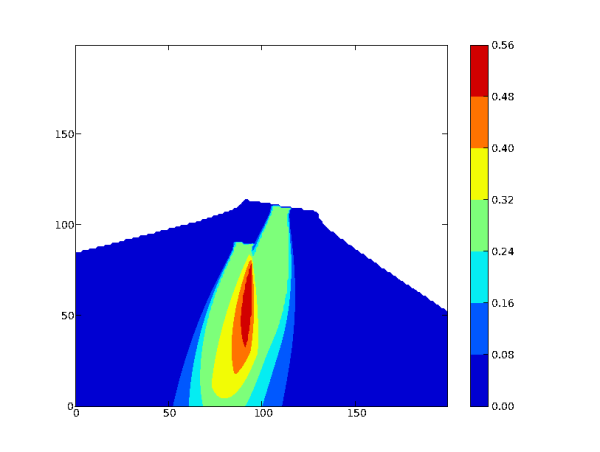
To visualize the concentration over the domain for the first situation and add a colorbar, use the following commands:

In [3]: contourf(d[0,0])
In [4]: colorbar()

You should obtain the figure shown below:

5-b) Gaussian Puff with Aerosol Species

You can go into the directory ~/TestCase/results/puff_aer/ and launch ipython from there, or either change directory from the ipython shell:

In [5]: cd ../puff_aer/

By doing that you ensure that you do not have to import atmopy again. However, when quitting ipython, you will be back in the directory from where it was launched.

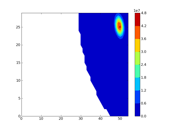
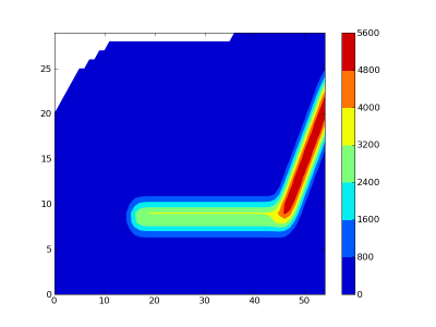
To visualize the ground concentration on the domain at time step t for meteorological situation i, you have to visualize the index (i-1) x Nt + t where Nt is the total number of time steps for one situation (here, Nt = 80). For example, the simulation time step 10 for the first situation corresponds to the index 10, for the second situation to the index 90, for the fourth situation to the index 250. To visualize the results at index i,use the command:

In [6]: d = getd(filename = 'aer1_0.bin', Nt=320, Nz=2, Ny=30, Nx=55)
In [7]: contourf(d[i, 0])

To visualize several time steps on the same figure, just use contourf several times. If you want to clear the figure, use the command clf(). Figure below gives an example of what you can obtain.

Puff
visualization at time steps 0, 9 and 30 for species aer1 and first diameter.
Third meteorological situation. Ground concentration in microgram/m^3.

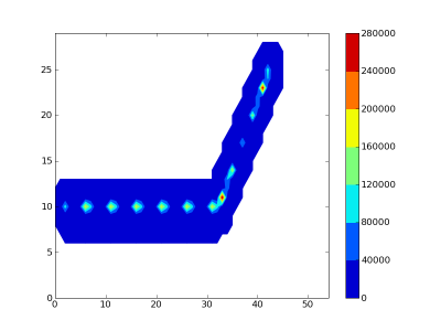
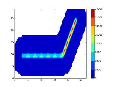
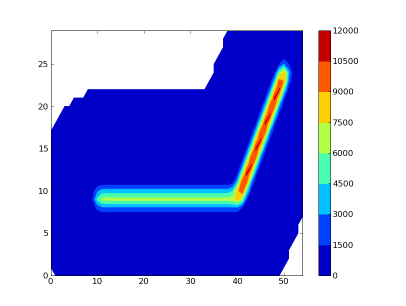
5-c) Gaussian Puff with Line Source

To visualize results, go to the directory ~/TestCase/results/puff_line/ and use the commands getd and contourf. This figure provides an example of what you can obtain: